Filter Banks and MFCC

Filter Banks

In a nutshell, a signal goes through a pre-emphasis filter; then gets sliced into frames and a window function is applied to each frame, afterwards, we do a Fourier transform on each frame(or more specifically a Short-Time Fourier Transform) and caculate the power spectrum, and subsequently compute the filter banks.

MFCC

To obtain MFCCs, a Discrete Cosine Transform is applied to the filter banks retaining a number of the resulting coefficients while the rest are discarded.

A final step in both cases, is mean normalization.

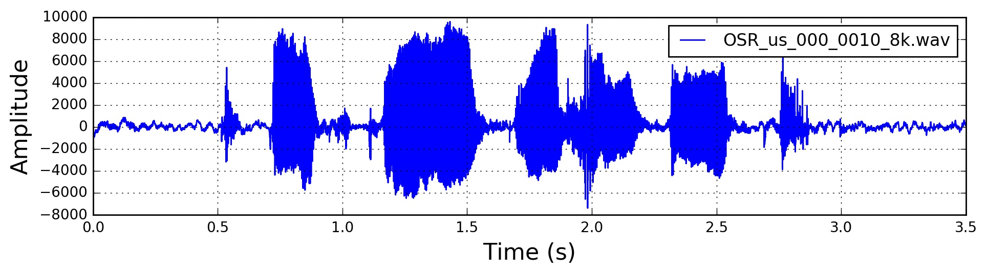
原始语音

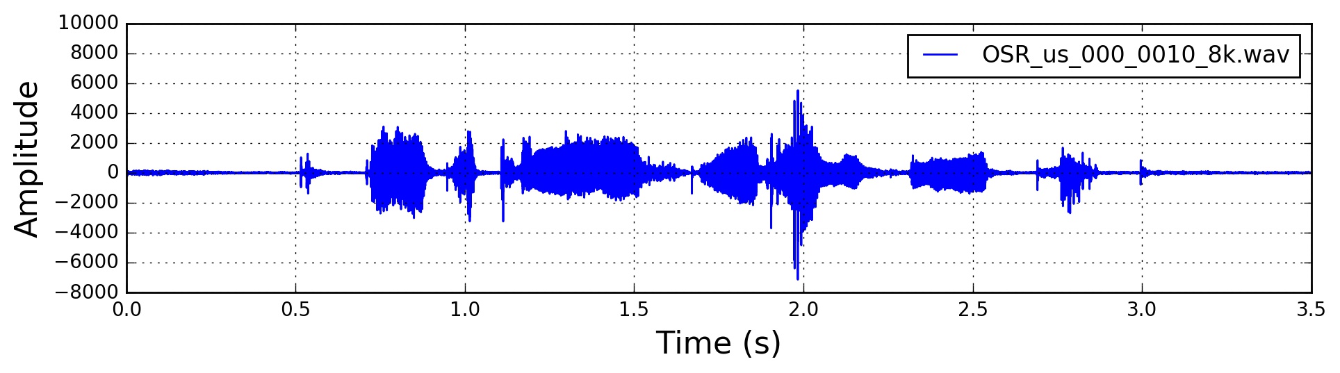
pre-emphasis

In order to amplify the high frequencies.

1. balance the frequency spectrum since high frequencies usually have smaller magnitudes compared to lower frequencies
2. Avoid numerical problems during the Fourier transfrom operation
3. improve the signal-to-noise ratio

2是pre-emphasis最modest的effect，1和3可以通过mean normalization 实现。

实现方法：

$$y(t) = x(t) - \alpha x(t-1)​$$

which can be easily implemented using the following line, where typical values for the filter coefficient ($\alpha$) are 0.95 or 0.97, pre_emphasis = 0.97

1

emphasized_signal = numpy.append(signal[0], signal[1:] - pre_emphasis * signal[:-1])

经过pre-emphasis的语音

framing

By doing a Fourier transform over this short-time frame, we can obtain a good approximation of the frequency contours of the signal by concatenating adjacent frames.

Typical frame sizes in speech processing range from 20ms to 40ms with 50% overlap between consecutive frames. Popular settings are 25ms for the frame size, and a 10ms stride(15ms overlap).

window

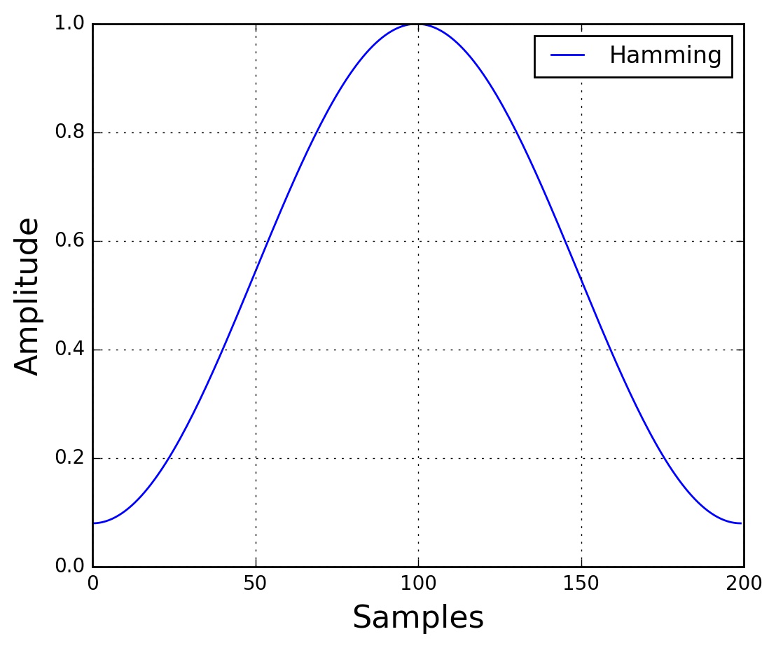
After slicking the signal into frames, we apply a window function such as Hamming window to each frame. A Hamming window has the following form:

$w[n] = 0.54 − 0.46 cos ( \frac{2πn}{N − 1} )$

where,$ 0≤n≤N−1$, $N$ is the window length. Plotting the previous equation yields the following plot:

There are several reasons why we need to apply a window function to the frames, notably to counteract the ssumption made by the FFT that the data is infinite and to reduce spectral leakage.

FFT算法只是对有限长度信号进行变换，有限长度信号相当于无限长信号和矩形窗的乘积，也就是讲这个无限长信号截短，对应频域的傅立叶变换是实际信号傅立叶变换与矩形窗傅立叶变换的卷积，当信号为截距后的频谱不同于它以前的频谱，例如，对于频率为fs的正弦序列，它的频谱应该只有在fs处有离散谱，但是在对它的频谱做了截短后，结果使信号的频谱不只在fs处有离散铺，而是在以fs为中心的频带范围内都有谱线出现，他们可以理解为从fs频率上泄漏出去的，这就是频谱泄漏

1

frames *= numpy.hamming(frame_length)

fourier-transform and power spectrum

We can now do an N-point FFT on each frame to calculate the frequency spectrum, which is also called Short-Time Fourier-Transform (STFT), where NN is typically 256 or 512, NFFT = 512; and then compute the power spectrum (periodogram) using the following equation:

$P = \frac{|FFT(x_i)|^2}{N}$

where, $x_i$ is the $i^{th}$ frame of signal $x$. This could be implemented with the following lines:

1
2

mag_frames = numpy.absolute(numpy.fft.rfft(frames, NFFT))  # Magnitude of the FFT
pow_frames = ((1.0 / NFFT) * ((mag_frames) ** 2))  # Power Spectrum

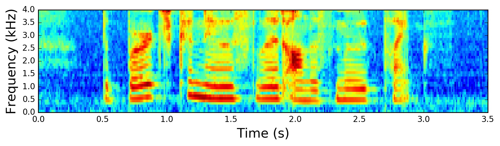
filter banks

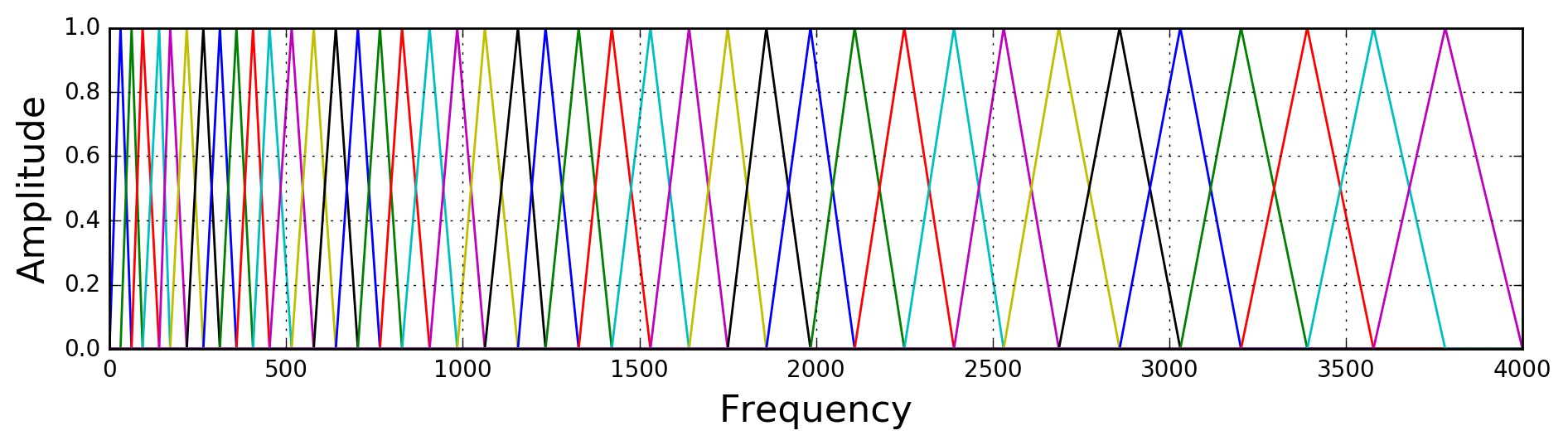
Final step: applying triangular filters, typically 40 filters, nfilt=40 on a Mel-scale to the power spectrum to extract frequency bands. The Mel-scale aims to mimic the non-linear human ear perception of sound, by being more discriminative at lower frequencies and less discriminative at higher frequencies.We can convert between Hertz (ff) and Mel (mm) using the following equations:

$m = 2595 \log_{10} (1 + \frac{f}{700})$

$f = 700 (10^{m/2595} - 1)$

1
2
3
4
5
6
7
8
9
10
11
12
13
14
15
16
17
18
19

low_freq_mel = 0
high_freq_mel = (2595 * numpy.log10(1 + (sample_rate / 2) / 700))  # Convert Hz to Mel
mel_points = numpy.linspace(low_freq_mel, high_freq_mel, nfilt + 2)  # Equally spaced in Mel scale
hz_points = (700 * (10**(mel_points / 2595) - 1))  # Convert Mel to Hz
bin = numpy.floor((NFFT + 1) * hz_points / sample_rate)

fbank = numpy.zeros((nfilt, int(numpy.floor(NFFT / 2 + 1))))
for m in range(1, nfilt + 1):
    f_m_minus = int(bin[m - 1])   # left
    f_m = int(bin[m])             # center
    f_m_plus = int(bin[m + 1])    # right

    for k in range(f_m_minus, f_m):
        fbank[m - 1, k] = (k - bin[m - 1]) / (bin[m] - bin[m - 1])
    for k in range(f_m, f_m_plus):
        fbank[m - 1, k] = (bin[m + 1] - k) / (bin[m + 1] - bin[m])
filter_banks = numpy.dot(pow_frames, fbank.T)
filter_banks = numpy.where(filter_banks == 0, numpy.finfo(float).eps, filter_banks)  # Numerical Stability
filter_banks = 20 * numpy.log10(filter_banks)  # dB

MFCC

It turns out that filter bank coefficients computed in the previous step are highly correlated, which could be problematic in some machine learning algorithms. Therefore, we can apply Discrete Cosine Transform (DCT) to decorrelate the filter bank coefficients and yield a compressed representation of the filter banks. Typically, for Automatic Speech Recognition (ASR), the resulting cepstral coefficients 2-13 are retained and the rest are discarded; num_ceps = 12. The reasons for discarding the other coefficients is that they represent fast changes in the filter bank coefficients and these fine details don’t contribute to Automatic Speech Recognition (ASR).

1

mfcc = dct(filter_banks, type=2, axis=1, norm='ortho')[:, 1 : (num_ceps + 1)] # Keep 2-13

One may apply sinusoidal liftering1 to the MFCCs to de-emphasize higher MFCCs which has been claimed to improve speech recognition in noisy signals.

1
2
3
4

(nframes, ncoeff) = mfcc.shape
n = numpy.arange(ncoeff)
lift = 1 + (cep_lifter / 2) * numpy.sin(numpy.pi * n / cep_lifter)
mfcc *= lift  #*

The resulting MFCCs:

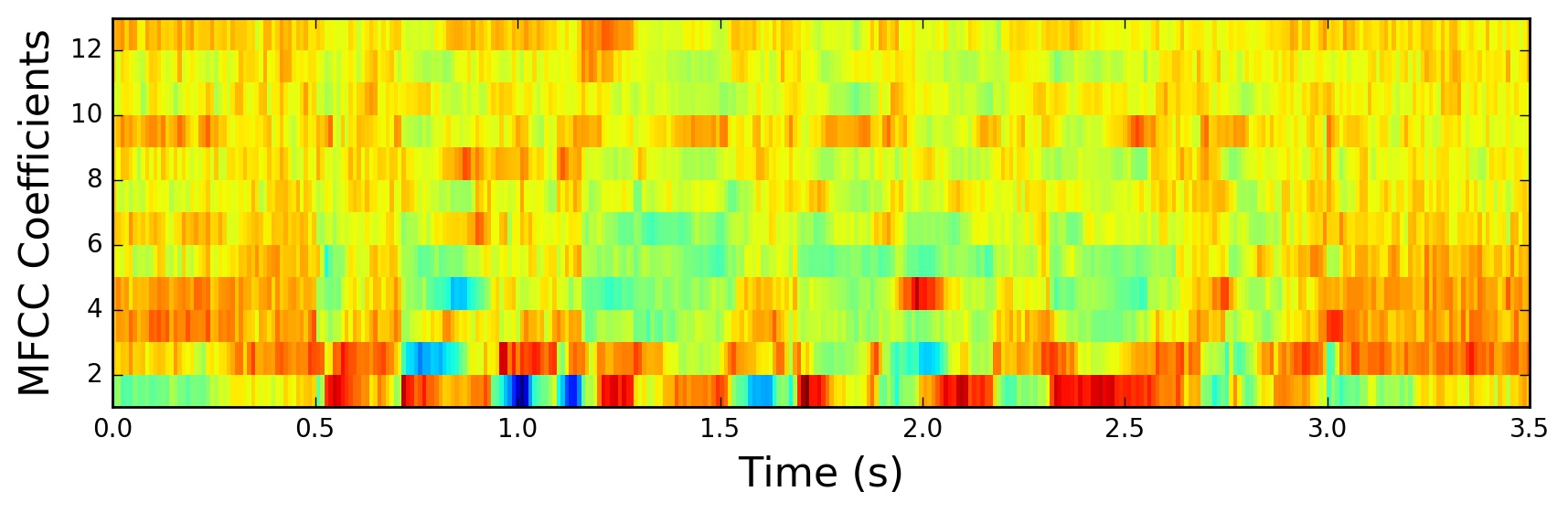MFCCs

Mean Normalization

As previously mentioned, to balance the spectrum and improve the Signal-to-Noise (SNR), we can simply subtract the mean of each coefficient from all frames.

1

filter_banks -= (numpy.mean(filter_banks, axis=0) + 1e-8)

The mean-normalized filter banks:

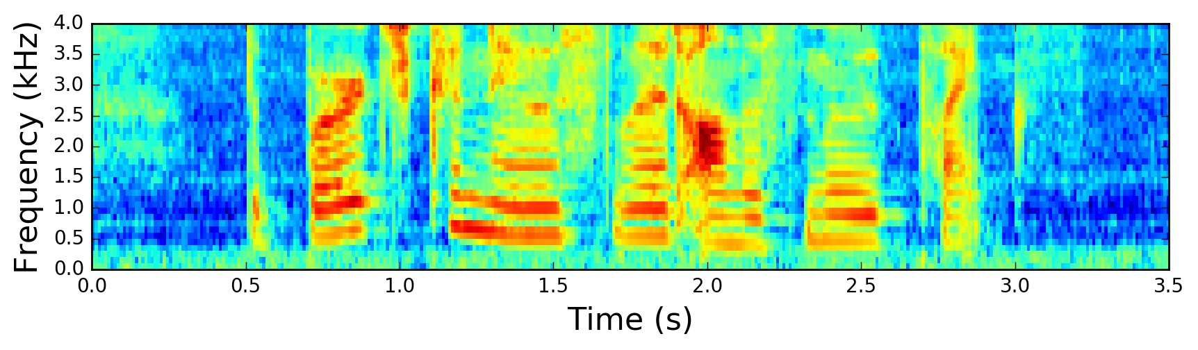Normalized Filter Banks

and similarly for MFCCs:

1

mfcc -= (numpy.mean(mfcc, axis=0) + 1e-8)

The mean-normalized MFCCs:

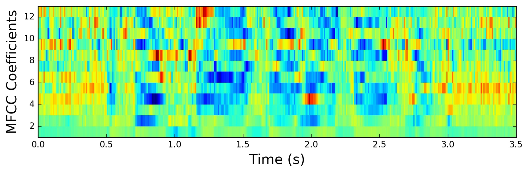Normalized MFCCs

Filter Banks vs MFCCs

To this point, the steps to compute filter banks and MFCCs were discussed in terms of their motivations and implementations. It is interesting to note that all steps needed to compute filter banks were motivated by the nature of the speech signal and the human perception of such signals. On the contrary, the extra steps needed to compute MFCCs were motivated by the limitation of some machine learning algorithms. The Discrete Cosine Transform (DCT) was needed to decorrelate filter bank coefficients, a process also referred to as whitening. In particular, MFCCs were very popular when Gaussian Mixture Models - Hidden Markov Models (GMMs-HMMs) were very popular and together, MFCCs and GMMs-HMMs co-evolved to be the standard way of doing Automatic Speech Recognition (ASR)2. With the advent of Deep Learning in speech systems, one might question if MFCCs are still the right choice given that deep neural networks are less susceptible to highly correlated input and therefore the Discrete Cosine Transform (DCT) is no longer a necessary step. It is beneficial to note that Discrete Cosine Transform (DCT) is a linear transformation, and therefore undesirable as it discards some information in speech signals which are highly non-linear.

It is sensible to question if the Fourier Transform is a necessary operation. Given that the Fourier Transform itself is also a linear operation, it might be beneficial to ignore it and attempt to learn directly from the signal in the time domain. Indeed, some recent work has already attempted this and positive results were reported. However, the Fourier transform operation is a difficult operation to learn and may arguably increase the amount of data and model complexity needed to achieve the same performance. Moreover, in doing Short-Time Fourier Transform (STFT), we’ve assumed the signal to be stationary within this short time and therefore the linearity of the Fourier transform would not pose a critical problem.

Conclusion

In this post, we’ve explored the procedure to compute Mel-scaled filter banks and Mel-Frequency Cepstrum Coefficients (MFCCs). The motivations and implementation of each step in the procedure were discussed. We’ve also argued the reasons behind the increasing popularity of filter banks compared to MFCCs.

tl;dr: Use Mel-scaled filter banks if the machine learning algorithm is not susceptible to highly correlated input. Use MFCCs if the machine learning algorithm is susceptible to correlated input.

topic identification

常规流程

1. speech is tokenized into words or phones by asr systems
2. standard text-based processing techniques are appplied to the resulting tokenlizations
3. Produce a vector representation for each spoken doument, typically a bag-of-wordds multinomial representation or a more compact vector give by probablilistic topic models
4. topic id is performed on the spoken document representations by supervised training of classifiers such as bayesian classifiers and svm

1-d peak

leetcode 162. Find Peak Element

A peak element is an element that is greater than its neighbors.

Given an input array nums, where nums[i] ≠ nums[i+1], find a peak element and return its index.

The array may contain multiple peaks, in that case return the index to any one of the peaks is fine.

You may imagine that nums[-1] = nums[n] = -∞.

bucket sort 总结

text classification

1. 如何hexo+next添加algolia搜索

   参考文章地址

2. jupyter需要加载安装好的虚拟环境

3. python编码规范

   ​ 等号一般在赋值的时候两边都要加空格，但是当’=’用于指示关键字参数或默认参数值时, 不要在其两侧使用空格.

   1. 1	Yes: def complex(real, imag=0.0): return magic(r=real, i=imag)

      ​

      避免在循环中用+和+=操作符来累加字符串. 由于字符串是不可变的, 这样做会创建不必要的临时对象, 并且导致二次方而不是线性的运行时间. 作为替代方案, 你可以将每个子串加入列表, 然后在循环结束后用 .join 连接列表. (也可以将每个子串写入一个 cStringIO.StringIO 缓存中.)

      1 2 3 4 5 6 7 8 9

      Yes: x = a + b x = '%s, %s!' % (imperative, expletive) x = '{}, {}!'.format(imperative, expletive) x = 'name: %s; score: %d' % (name, n) x = 'name: {}; score: {}'.format(name, n) No: x = '%s%s' % (a, b) # use + in this case x = '{}{}'.format(a, b) # use + in this case x = imperative + ', ' + expletive + '!' x = 'name: ' + name + '; score: ' + str(n)

4. 英语积累

   1. Tensor and Function are interconnected and build up an acyclic graph

word2vec 总结

Image Pre-Processing